Table of Contents
Go to ⇒ [ PI ] - [ 6ka ] - [ 21ka ] - [ LM ] - [ 8.2ka ] - [ LI ] - [ Plio ]
21ka Experimental Design
Make sure you use the final version of the 21ka BC!
Boundary conditions
Summary of 21ka boundary conditions
| PMIP3 | Minimum solution | |
|---|---|---|
| Orbital parameters | [ ecc = 0.018994 ] - [ obl = 22.949° ] - [ peri-180° = 114.42° ] | |
| Date of vernal equinox | March 21 at Noon | |
| Trace gases | [ CO2 = 185 ppm ] - [ CH4 = 350 ppb ] - [ N2O = 200 ppb ] - [ CFC = 0 ] - [ O3 = same as PI ] | |
| Aerosols | Same as PI (see Dust forcing note below) | |
| Solar constant | 1365 W/m2 | As in PI |
| Vegetation | Interactive | See specific note below |
| Ice sheet | Revised ICE5G???? (provided) * | |
| Topography and coastlines | From ???? (provided) * | minimum changes (see note below) |
| River outflow | Modified according to a river pathway map (provided) | Same as PI |
| Ice sheet ice stream | add excess LGM freshwater (see below) | Same as PI |
| Mean ocean salinity | ??? -1PSU everywhere ??? |
* see discussion on the ice-sheet
Please use the discussion panel to comment this table!
Ice-sheet
The ice sheet to be used for PMIP3/CMIP5 experiments is still under discussion. Click on the link below to have access to the ongoing propositions and discussions
Vegetation
The vegetation should be treated as in the CMIP5 PI experiment. The reason is that in CMIP5 we test the version of the model used for future climate projections. Since OA and ESM models will be considered, depending on the model used the vegetation will be
- prescribed to PI (which means both vegetation types and LAI are prescribed )
- Prescribed to PI with interactive LAI (models with interactive carbone cycle, but no vegetation dynamics)
- Computed by the model (models with dynamic vegetation)
There are still questions concerning the possibility to have a 6ka reconstructed vegetation from a combination of model output and data analyses that could be used for sensitivity experiments. Please tell if you are interested by such a map and what would be the best variables (pft?) that should be provided (see comment from B. Otto-Bliesner in the discussion panel).
For Earth System Models with interactive carbon cycle
The simlations are forced by CO2 concentrations. Please use the same protocol as in CMIP5 to store the carbon fluxes and the variables needed for PCMIP (see list here)
Insolation
Note that insolation should follows PMIP requirements. Please check it carefuly using the following tables (LGM insolation tables)
River outflow
The river pathways and basins should be at least adjusted so that fresh water is conserved at the Earth's surface: care should be taken that rivers reach the ocean (due to the lower sea level at LGM, some river mouths have to be displaced towards the coast).
Ice-sheet mass balance
It is advised to ensure a closed fresh water balance at the Earth's surface: snow accumulating on the ice-sheets should be redistributed to the oceans, either globally or in the adjacent oceans.
Dust forcing
Some ESM have interative aerosols. In that case compute dust and associated forcing online, as in PI. If this is not the case then the recommendation is to keep dust and aerosols as in PI (I.E no change for 21 ka).
Initial conditions
Additional information
Siberia winter palaeotemperatures
The following maps has been provided by Alexander Kislov and Yurij Vasil'chuk (Moscow State University)

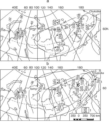
Siberia winter palaeotemperatures, reconstructed by δ18O in ice wedges formed 30-25 (a) and 22-14 (b) ka BP

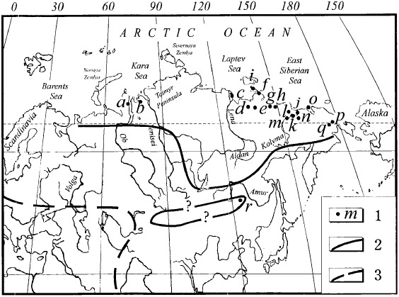
Map of northern Eurasia showing localities mentioned in text where 14C dated syngenetic ice-wedges formed during the Late Pleistocene.
Legend: (1) localities of 14C dated sequences; (2) southern boundary of modern and Late Pleistocene syngenetic ice-wedges; (3) southern boundary of Late Pleistocene palaeopermafrost zone.
[ PMIP3 Wiki Home ] - [ Help! ] - [ Wiki syntax ] - [ Top ]

Discussion
Ice-sheet mass-balance redistribution is non-trivial. Even if the ice-sheet is assumed to have 0 net mass-balance change, regional discharge will vary. Ie part of the ice-sheet can be growing, another part shrinking resulting in spatially heterogenous discharge to the oceans. Combined drainage/ice-sheet/isostasy modelling can resolve this and create a self-consistent routing map.
A related issue is iceberg versus meltwater discharge. Glaciological models approximately resolve this (we lack well constrained calving models, so emphasis on the “approximate”). Is it worth considering different treatment of freshwater versus ice-berg discharge wrt when mixing can occur in the ocean?
Topography and coastlines need to be a part of the self-consistent ice-sheet/topography package.
A vegetation map for 21ka reconstructed from a combination of model output and data analyses would be very useful for modeling groups that will not be using interactive vegetation in their PI and 20th century runs. We could query groups on the best format. For CCSM, a pft vegetation map would be best.
We would like to add in this Table (21 ka boundary conditions) the new line “PERMAFROST DISTRIBUTION”. Apart from, we can discuss the scale of Arctic ocean regression during the 21 ka BP as at that time in Yamal, Gydan and Timyr Peninsulas marine terraces were formed. It means that ocean level was high as today. We have the detailed maps of stable isotope distribution in permafrost at this time so we have good instrument for winter temperature reconstruction.
Professors Alexander Kislov and Yurij Vasil’chuk (Moscow State University)
As example, we present two maps, containing the mean January temperature reconstructed based on the signal of the δ18O in ice wedges Professors Alexander Kislov and Yurij Vasil’chuk (Moscow State University)
(unfortunately, maps, probably, can not be represented!)
Fig.1. Sibiria winter palaeotemperatures, reconstructed by δ18O in ice wedges formed 30-25 (a) and 22-14 (b) ka BP.